NANSLO REMOTE LAB ACTIVITY

 

SUBJECT SEMESTER: XXXXXXXXXXXXXXXXXXXXX

TYPE OF LAB:  Spectroscopy

 

 

 

 

 

 

TITLE OF LAB:  Beer-Lambert Law

 

Beer-Lambert Law NANSLO Lab Activity in Word format last updated May 7, 2014

 

Lab format: This lab is a remote lab activity.

 

Relationship to theory (if appropriate):  This activity quantitatively relates the concentration of a light-absorbing substance to the absorbance of light.

 

Instructions for Instructors:  This protocol is written under an open source CC BY license. You may use the procedure as is or modify as necessary for your class.  Be sure to let your students know if they should complete optional exercises in this lab procedure as lab technicians will not know if you want your students to complete optional exercise.

 

Instructions for Students:  Read the complete laboratory procedure before coming to lab.  Under the experimental sections, complete all pre-lab materials before logging on to the remote lab, complete data collection sections during your on-line period, and answer questions in analysis sections after your on-line period.  Your instructor will let you know if you are required to complete any optional exercises in this lab.

 

Remote Resources:  Primary - UV/Vis Spectrometer; Secondary - Cuvette Holder

 

CONTENTS FOR THIS NANSLO LAB ACTIVITY:

 

Learning Objectives

Background Information

Equipment
Pre-lab Assignment

Experimental Procedure

Preparing or the NANSLO Lab Activity

 

LEARNING OBJECTIVES:

 

After completing this laboratory experiment, you should be able to do the following things:

 

1. Measure and analyze the visible light absorbance spectrum of a standard NiSO₄ solution to determine the maximum wavelength of absorbance (λ_max).
2. Measures the absorbance of several standard NiSO₄ solutions.
• Calculate the concentrations of these standard solutions using information provided by the Laboratory Technician.
3. Create tables to display observations.
4. Construct a standard curve for the standard solutions. Find the relationship between absorbance and concentration for NiSO₄. 
5. Measure the absorbance of an unknown concentration of the NiSO₄ solution.
6. Calculate the concentration of the unknown NiSO₄ solution using the standard curve that you derived.

 

 

BACKGROUND INFORMATION:

 

Visible light represents only a very small part of the electromagnetic spectrum. Visible light consists of light having wavelengths from about 3.8 x 10^-7m to 7.8 x 10^-7 m (380 nm to 780 nm).

Many substances interact with electromagnetic radiation in the visible and ultraviolet regions of the spectrum.  Substances that have color absorb some wavelengths from the visible region of the spectrum and reflect others. The energies associated with photons of visible and ultraviolet light are in the same range as energies required to promote outer level (valence shell) electrons to higher energy level in many substances.

E = hν is the difference in energy between the ground state and the excited state. When light of the appropriate wavelength impinges on a substance, it may be absorbed by promoting an electron to a higher energy level. This happens in the visible and ultraviolet regions of the spectrum.

 

The energy of a photon of electromagnetic radiation is given by the relationship:   E = hν where E = energy in joules, ν = frequency in cycles per second, and h = Planck’s constant =  6.62607 x 10-34 J•s The relationship between wavelength and frequency of electromagnetic radiation is:  λν= c where  λ = wavelength in meter and c = 2.996 x 108 m/s, the speed of radiant energy in a vacuum

 

In making measurements of the amount of radiant energy absorbed or transmitted by a sample, we use a blank so that the change in absorbance of the sample holder and the solvent can be factored out. That is, a blank containing all substances that will be in the sample, except the one under investigation, is placed in the spectrophotometer, and a measurement is taken so that we know how much light is absorbed by everything except the substance we are trying to investigate.

The absorbance of a solution can be related to the concentration of the absorbing species in the solution. This relationship is called the Beer-Lambert law, after Augustus Beer (a German physicist) and Johann Lambert (a Swiss physicist), but is commonly referred to as Beer’s Law, although it has nothing to do with beer.  The Beer-Lambert Law can be expressed as:

 

A = abc where A = Absorbance (unitless); a = molar absorptivity (molarity-1∙cm-1), which is a constant for the absorbing species,  b = path length, or thickness of the absorbing layer of a solution (cm), and c = concentration of the solution (molarity).

 

Beer’s law tells us that the absorbance of a particular species is directly proportional to the concentration of the absorbing species. The measurement of a blank, as described above, allows us to factor out the effect of the solvent, cell walls and cell length.

So A = abc, and if a and b are constant for any given species and cell length, we can see that the absorbance of a solution is directly proportional to the concentration of the absorbing species. Because the absorbance of a solution is easy to measure, this technique is frequently used to measure concentrations of unknown solutions, and this is what you will be doing in this experiment.

 

There are many sources of noise, or uncertainty, in any experimental measurement that you will ever make.  The goal of any scientific data collection is to gather data with as little noise as possible, although it can never be totally eliminated.  For example, using a spectrometer with fiber optic light transfer, as you will do in this lab activity, has noise in its measurements due to the inconsistencies in the fiber optics, interference between the light and the sample being measured,

inefficiencies in the detector, etc.  Most of this noise is random, meaning that it has the same probability of resulting in a measurement that is too high as it does in a measurement that is too low.  When noise is random, it can be minimized by averaging multiple measurements.  In a spectrometer such as this one, there are two methods of averaging measurements.  One method is the use of “boxcar averaging,” and the other method is to average multiple complete spectra.

Boxcar averaging is a smoothing method by which multiple points on a curve are averaged into one point.  This reduces the overall number of points in the curve, but it averages out some of the random noise in those points.  One must be careful not to average too many points on the curve together, because the more points you average in each “boxcar” the less information there is in that curve.  For example, in the extreme case where you averaged ALL the points on the curve, you would end up with just one point, which is not very useful.  Essentially, you specify how many points you want in the averaging function.  Let’s say that you specify two points for the boxcar average, and let’s further assume that the curve you are smoothing has 1000 points in it.  The process works like this:

• Points #1 and #2 are averaged to become a single point which we will call NewPoint #1.
• Then, the ORIGINAL point #2 is averaged with the ORIGINAL point #3 to become the second point in the new curve which we’ll call NewPoint #2. 
• The process continues, with the boxcar moving ahead one point at a time until all the original points are averaged to become NewPoints in the smoothed curve.
• The original 1000 points are turned into 999 NewPoints and you have a slightly smoother curve.

Figure 3 below illustrates how this process would proceed for a small curve of 50 original points.  The “y” curve is the 50 original points and the “y-box” curve is the 49 “new” points.

 

Figure 1:  Example of Boxcar averaging.

 

The other type of averaging is to average the entire curve.  The spectrometer will collect one entire spectrum about once per second.  The spectrum consists of many thousands of points, and each time a spectrum is collected, these points are slightly different (due to random noise).  If you average two spectra together, you reduce the noise by a factor of √2.  If you average three spectra, you reduce the noise by a factor of √3, etc.  Of course, the more spectra you average, the longer it takes to get a result, so there is a balance between decreasing noise and collecting data in a reasonable amount of time.

 

EQUIPMENT:

 

• Paper
• Pencil/pen
• Computer with Internet access
  
  

PRE-LAB ASSIGNMENT:

 

1. Why are we measuring the absorbance of various samples in this lab activity? 
2. What are the sources of noise in the measurements you will be making? 
3. How can you reduce the noise in your measurements?  
4. What two factors must you balance when deciding how to collect your data? 
5. Read the procedure below and ask your Instructor if you need any clarification on any of the steps.

 

EXPERMENTAL PROCEDURE:

 

Once you have logged on to the remote lab system, you will perform the following laboratory procedures.  See Preparing for the Beer-Lambert Law NANSLO Lab Activity below. 

Once you have logged on to the Remote Lab, you will perform the following Laboratory procedures.  Feel free to “play around” a little bit and explore the capabilities of the equipment before you start the actual procedure.

 

1. Turn on temperature controller.  Ensure the temperature of the system is adjusted to 25.0 degrees C. 
2. Ensure the spectrometer’s light source is turned off.   
3. Store a Dark Spectrum.  
4. Ensure that cuvette 0 (the reference sample) is selected.  
5. Turn on the light and you will see the spectrum of the light source. 
6. Play around with the Boxcar Width and # Spectra to Average to get the least noisy spectrum that you can. 
7. Store the Reference spectrum. 
8. Ask the Lab Tech for information about the standard NiSO4 solutions.  You will use this information to calculate the concentration of each standard solution (during data the analysis portion of the activity). 
9. Select one of the NiSO4 standards (cuvettes 1 through 4) in the Qpod.  
10. View the Absorbance Spectrum. 
11. Determine the location of λmax. 
12. Record the Absorbance of the NiSO4 sample at λmax.  Each student in the group must write the measurement down for later use. 
13. Repeat step 9 for all remaining samples, including cuvette #5 which contains the unknown concentration of NiSO4. 
14. Another student should take control of the interface and repeat the process starting at step 2. 
15. After each student has collected a complete set of data (and everyone has recorded each data set), you can log out of the lab and work on the data analysis portion.  If you have time left in your scheduled lab period, you can continue working with your lab partners to analyze the data.

 

Data Analysis (to be done offline if necessary):

 

Plot a standard graph using the concentration and Absorbance values for the standard solutions.  Plot Concentration on the X-axis and Absorbance values on the Y-axis.  Draw a best-fit line going through the origin.  From the Absorbance of the unknown solution, you can calculate the concentration of the unknown solution using the line equation of the standard curve.

 

In Excel, the best-fit line and its equation can be determined by this method:

 

1. Insert a scatter plot of the data, making sure that absorbance is on the y axis and concentration is on the x axis. If they are switched, then delete the graph, change the positions of the absorbance and concentration columns and insert the scatter plot graph again.
2. Right-click one of the data points on the graph and select Add Trendline.
3. Make sure “Linear” is selected and check the box to set the intercept to zero and also the one to display the equation on the chart.
4. You will now have the best-fit line and the equation for that line.  You can use this line equation to calculate the concentration of the unknown NiSO₄ solution

Questions (show all necessary calculations):

 

1. Why do you have to first take an absorbance measurement of a cuvette filled with distilled water?  Why does this measurement have to be subtracted from the measurements of the NiSO4 samples?
2. Why didn't we just measure one or two samples with known concentrations of NiSo₄?
3. How many significant digits can you report in the concentration of the unknown sample?  What limits the number of significant digits in this result?
4. What is the energy, in Joules, of one photon of light at A_max?
5. Use Figure 1 to determine what color light is being absorbed for A_max.
   
   
                                    Figure 1 - Visible portion of EM Spectrum
   
   
6. Figure 2 demonstrates the relationship between absorbed and reflected colors of light.  Absorbed is opposite of reflected on the wheel.  For example, if a substance absorbs orange light, it will reflect blue light, and therefore appear blue.  Compare the color of the NiSO4 solution to the color of the light it absorbs.  Does it agree with the color wheel?  What can you deduce from this?
   
                                          
                  Figure 2 - By Sakurambo at English Wikipedia [GFDL (http://www.gnu.org/copyleft/fdl.html)
                  or CC-BY-SA-3.0 (http://creativecommons.org/licenses/by-sa/3.0/)] via Wikimedia Commons                                     
   
   
7. If a chemical solution was primarily orange in color, approximately what wavelength would you expect λmax of the absorbed light to be?  Why?

 

PREPARING FOR THE BEER-LAMBERT LAW NANSLO LAB ACTIVITY:

 

Read and understand the information below before you proceed with the lab!

  

Scheduling an Appointment Using the NANSLO Scheduling System

 

Your instructor has reserved a block of time through the NANSLO Scheduling System for you to complete this activity. For more information on how to set up a time to access this NANSLO lab activity, see www.wiche.edu/nanslo/scheduling-software.  

 

Students Accessing a NANSLO Lab Activity for the First Time

 

You must install software on your computer before accessing a NANSLO lab activity for the first time. Use this link to access instructions on how to install this software based on the NANSLO lab listed below that you will use to access your lab activity – www.wiche.edu/nanslo/lab-tutorials.

 

1. NANSLO Colorado Node -- all Colorado colleges.
2. NANSLO Montana Node -- Great Falls College Montana State University, Flathead Valley Community College, Lake Area Technical Institute, and Laramie County Community College.
3. NANSLO British Columbia Node -- Kodiak College.

 

Using the UV/Vis Spectrometer and Cuvette Holder for a NANSLO Lab Activity

 

We've provided you with two ways to learn how to use this equipment for this NANSLO lab activity:

 

1. Read these instructions
2. View this short video.
   
   
   
   NOTE:  The conference number in this video tutorial is an example.  See "Communicating with Your Lab Partners" below to determine the toll free number and pin to use for your NANSLO lab activity.
   
   

LAB INTERFACE INSTRUCTIONS FOR ABSORBANCE APPARATUS

 

The Remote Web-based Science Lab (RWSL) spectrometer is controlled remotely by using a web interface as shown below.  This lab interface allows you to control every function of the spectrometer just as if you were sitting in front of it. 

 

The equipment control software shown below is written using the LabVIEW software from National Instruments. The user interface is presented as a LabVIEW control panel which will be referred to as the lab interface for the remainder of the document.

 

Figure 4: Spectrometer lab interface for emission spectroscopy lab

 

COMMUNICATING WITH YOUR LAB PARTNERS

 

As soon as you have accessed this lab interface, call into the toll free conference number shown on the control panel to communicate with your lab partners and with the Lab Technicians.  Use the PIN code noted to join your lab partners.  Only one person can be in control of the equipment at any one time so talking together on a conference line helps to coordinate control of the equipment and creates a more collaborative environment for you and your lab partners.

 

 

GAINING CONTROL OF THE ABSORBANCE APPARATUS

 

Right click anywhere in the gray area of the lab interface and choose “Request Control of VI” from the dialogue box that appears when multiple students are using the spectrometer at the same time,.  After you request control, you may have to wait a short time before you actually receive control and are able to use the features on this lab interface.

 

Figure 5:  Take control of the lab interface by right clicking
and selecting "Request Control of VI."

 

RELEASING CONTROL OF THE ABSORBANCE APPARATUS

To release control of the spectrometer so that another student can use it, right click anywhere in the gray area of the lab interface and choose "Release Control of VI" from the dialogue box that appears.

 

Figure 6: Release control of the lab interface by right clicking
and selecting "Release Control of VI."

 

LAB INTERFACE CONTROLS FOR THE SPECTROMETER, QPOD, AND QPOD TEMPERATURE CONTROLLER

 

This lab interface provides controls for three pieces of equipment.  More detailed instructions are provided below on using the controls for each piece of equipment. 

 

1. Spectrometer analyzes the light absorbed in a sample and visually displays the absorbance spectrum of the sample, the absorbance value, and the wavelength at λ_max.   Spectrometer controls are available when the “Spectrometer” tab of the lab interface is selected.
   
   
2. Qpod is a carousel that holds six cuvettes.  A selected cuvette is rotated into place so that light can be shined through it in order to measure absorbance.  Qpod controls are available when the “Cuvette Holder (Temp Control)” tab is selected and then the “Cuvette Selection” tab is selected.
   
   
3. Qpod temperature controller controller raises the temperature of the sample in the cuvette placed inside of it based on the temperature selected.  The temperature controller is available when the “Cuvette Holder (Temp Control)” tab is selected and then the “Temp Control Display” tab is selected.

 

Figure 8 shows the equipment configuration for this lab.  The light path is indicated with yellow arrows.  Some of the fiber optic cabling that the light flows through is not visible in the photo.  The light is produced by a Xenon strobe inside the spectrometer.  The light passes through a fiber optic cable into one side of the Qpod where it then passes through whatever sample is inside the Qpod.  The light next enters a fiber optic cable on the other side of the Qpod and is returned to the sensing unit in the spectrometer.  The spectrometer measures how much light is passed and how much light is returned, thus determining how much light is absorbed in the sample.

 

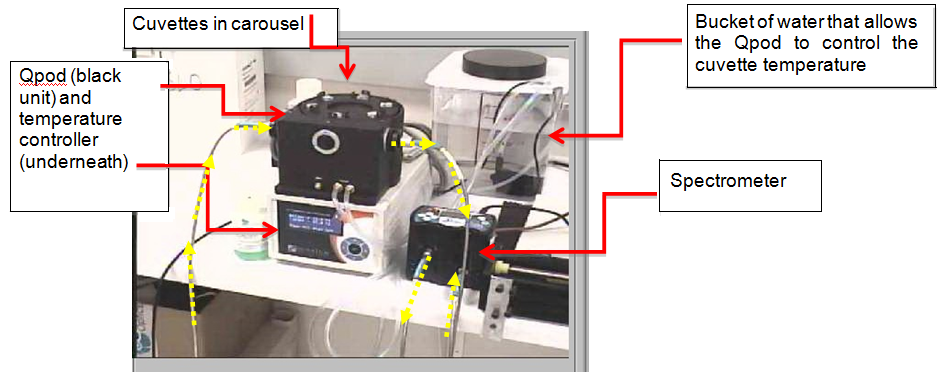
Figure 7:  Experimental apparatus (Spectrometer, Qpod and Cuvettes)
for Beer-Lambert law NANSLO lab activity.

 

 

SPECTROMETER CONTROLS

 

When the “Spectrometer” tab is selected, controls are available for the spectrometer. 

 

To activate the spectrometer to start the data feed, click the "Start" button on the far left portion of the lab interface. The button will now turn yellow and say “Pause”.

 

Figure 8:  After clicking on the "Start" button, it turns to a "Pause" button.

 

The Image View Window on the upper right-hand side of the screen displays the real-time video feed from a digital camera focused on the equipment used for this NANSLO lab activity based on the Camera Preset selected. 

 

The controls in the lower left hand corner of this screen allow you to capture lab data generated by the spectrometer.  See Figure 9. 

 

Figure 9:  Controls for the spectrometer.

 

ZOOMING IN AND OUT ON THE SPECTRUM GRAPH ON THE LEFT-HAND SIDE OF THE
SPECTROMETER SCREEN

 

You will need to “zoom out” on the spectrum window to view the entire spectrum properly.  Here’s how to zoom out and in on the spectrum.

 

Click on the center button at the lower right of the graph, shown below in Figure 10.

                                 

Figure 10:  Click button to access other options.

 

This brings up a small sub-menu containing other buttons.  The only two buttons that are useful to you are the left-most buttons in the top and bottom rows.  Select the left-most button in the bottom row to view the entire spectrum. 

 

Figure 11:  Spectrum Zoom Out Button

 

Select the left-most button in the top row to select specific parts of the spectrum to “zoom in” on and view more closely (see Figure 12).  After clicking this button, your mouse turns to a magnifying glass.   Use your mouse (hour glass) to select a portion of the spectrum to inspect more closely by holding down your mouse button and drawing a box around the area of interest.  Be sure you draw the box so that it includes some area past the top of the peak you are interested in or else it will chop off the top of it in the viewing window. The enlarged image of that area will appear in the spectrum window.  If you accidentally zoom in too far or on the wrong part of the spectrum, use the zoom out button shown in Figure 11 and start over again.

 

Figure 12:  Spectrum Zoom In Button

 

QPOD CONTROLS

 

To access the Qpod Controls, select the “Cuvette Holder (Temp Control)” tab and then the “Cuvette Selection” tab.  The Qpod controls are used to select a sample to analyze and collect data on.  The sample contained in each cuvette is determined based on the lab being performed.  A cuvette is a small laboratory vessel used to hold the sample.  All of our cuvettes have a path length (distance that the light travels through them) of 1.00 cm.  (Photo from http://cuvette.net/).

 

Using Camera Preset 4, zoom in to actually see the Qpod carousel rotate.

 

To select the Reference Sample (if not already selected,) you would use the back and forth arrows until “0” is displayed in the “Selected Cuvette” field or click the “Re-set to Reference” button. 

 

For all other selections, you would use the back and forth arrows until the sample of interest is displayed in the “Selected Cuvette” field, e.g. “3.”  Your lab procedure will provide more detail on the samples to select.

 

Figure 13:  Accessing the Qpod Carousel Controls

 

QPOD TEMPERATURE CONTROLLER CONTROLS

 

To access the Qpod Temperature Controller, select the “Cuvette Holder (Temp Control)” tab and then the “Temp Control Display” tab. 

1. First select the “Temperature Controller” button to turn on the heater.
2. First select the “Temperature Controller” button to turn on the heater.
3. View the current temperature in the “Current Temperature *C” area and wait until it reaches the set temperature before proceeding to college data.

Using Camera Preset 2, zoom in to actually see the temperature on the Qpod Temperature Controller.

 

Figure 14:  Accessing the Qpod Temperature Controller Controls

 

CAMERA PRESETS AND PAN-TILT-ZOOM CONTROLS AVAILABLE FOR
SPECTROMETER, QPOD, AND QPOD TEMPERATURE CONTROLLER

 

Several camera preset positions have been programmed for use with this lab interface.  Hovering over the gray area where the buttons are will give you a pop-up menu that describes where each preset is assigned to.  Each Camera Preset is set to focus in on a specific area.  Preset 1, for example, zooms in on a portion of experimental setup, Preset 2 on the temperature control, Preset 3 on the sample in the cuvettes; and Preset 4 on the carousel holding the cuvettes.

 

Figure 15:  Absorbance NANSLO lab activity camera presets.

 

Figure 16 shows the Pan-Tilt-Zoom Controls available.  The four arrows are used to pan and tilt allowing you to move the camera right to left and up and down.  The two zoom buttons allow you to zoom in to see a closer look at the equipment or zoom out to view more of the room.

 
 

Figure 16: Pan, tilt and zoom capabilities.

 

STEPS IN PERFORMING YOUR LAB ACTIVITY

 

Storing the Dark Spectrum Before Turning on the Spectrometer Light

To establish a level of baseline “noise” in the instrument, which will automatically be subtracted out later in the process, you need to store the “dark spectrum” which is merely a measurement of what the spectrometer is measuring when there is no light present.  With the “Spectrometer” tab is selected, click on the “Store Dark” button.  There will be no indication that anything happened, so if you’re not sure you clicked this button, just click it again – you won’t hurt anything by storing another dark spectrum.  See Figure 17. 

 

Figure 17:  Storing the Dark Spectrum.

 

Turning on the Spectrometer Light

Now turn on the spectrometer’s light source by clicking the “Light” button.  The button turns green.   You should now see a spectrum (left-hand window of this lab interface) that looks similar to the one shown in Figure 18. 

 

Figure 18:  Turning on the spectrometer light. 

 

Turning on the Qpod’s Temperature Control System

 

Turn on the Qpod Temperature Controller heating unit.  Several steps must be performed to complete this step.

1. Select the “Cuvette Holder (Temp Control)” tab.  
2. Select the “Temp Control Display” tab if not selected by default. 
3. Select the “Temperature Control” button.  It will turn green and display “On” when selected.  
4. In the “Set Temperature *C” field, ensure that it is set to 25.00 °C, which is the standard temperature for most Absorbance measurements, or whatever temperature is indicated in your lab procedure. 
5. Watch the temperature curve for a few minutes to ensure that the temperature of the Qpod is adjusted to 25.00 °C +/- 0.05 °C. 
   
   

Note that if you have selected Camera Preset 2 you can see the temperature on the Qpod.

 

Figure 19:  Setting the Qpod temperature. 

 

Selecting the Reference Sample

 

The “Cuvette Holder (Temp Control) tab is currently selected.  Select the “Cuvette Selection” tab.  As mentioned above, the Cuvette Selection tab allows you to rotate the carousel that holds the six cuvettes.  They are numbered 0 through 5. You will use this tab to select each sample that will be used for this lab activity. 

 

For now, make sure that the “reference sample” is selected:  “Cuvette 0 = Reference Sample.”  The reference sample is a cuvette full of distilled water.   If the reference sample is not selected, either use the arrows to navigate to that cuvette or select the “Reset to Reference” to return to Cuvette 0. 

Note that if Camera Preset 4 has been selected, you can see the carousel on the Qpod move.

 

Figure 20:  Selecting the Reference Sample.

 

Storing the Spectrum for the Reference Sample

Next, select the “Spectrometer” tab.  Click the “Store Ref” button to collect and store the spectrum of the “reference sample”.  A spectrum where light is being absorbed by the cuvette and by water is stored and allows it to be subtracted out from your later sample measurements, thus allowing you to measure the Absorption of light that is only due to the material you are interested in (NiSO₄ in this experiment).  

 

Figure 21:  Storing the spectrum for the Reference Sample.

 

MEASURING THE ABSORBANCE OF NICKEL (II) SULFATE

 

Background:  There are several standard NiSO₄ solutions that you will measure the absorbance of.  This range of concentrations was chosen because the Absorbance is directly proportional to the concentration (obeys Beer’s law) in this concentration range. By plotting Absorbance on the y-axis and concentration of NiSO₄ on the x-axis, you will draw a best-fit straight line (which is called the “standard curve”) passing through the origin.  When you measure the absorbance of the sample, you must do so at a single wavelength.  This is called the λ_max, and corresponds to the tallest peak in the absorbance spectrum.  It is important that this wavelength be the one at which the sample absorbs light the most strongly, because this results in the most favorable signal-to-noise ratio and gives an absorbance measurement with the least amount of uncertainty. 

 

Selecting the Standard:  Select the “Cuvette Holder (Temp Control)” tab and then the “Cuvette Selection” tab.  Select one of the standard solutions (cuvettes 1 – 4).  Tell the lab tech which cuvette you have selected, and you will be provided information that will allow you to calculate the concentration of the standard solution selected.  You will do this for each standard solution. 

 

Viewing the Spectrum of the Selected Standard:  Select the “Spectrometer” tab.  With the cuvette containing NiSO₄ in the Qpod, select the “Show Absorbance Spectrum” button.  Notice that the line on the absorbance spectrum may look flat.  If so, you need to adjust the scale so you can see it. 

 

Figure 22:  Selecting the “Show Absorbance Spectrum” button.

 

Zoom out to view the whole spectrum (see Figure 11 on zooming out.) You will see a peak that is the absorbance peak and noise on either side of it where we have run out of light intensity.  Use spectrum “zoom in” tool to look at the tallest peak more closely.

 

Identifying λ_max:    λ_max is the tallest peak in the Absorbance Spectrum.  You only need to identify λ_max once for a chemical.  No matter how many different concentrations of that chemical you measure, λ_max is always the same.  So, you don’t need to adjust the cursor location after you have it set.

 

You can ignore the noisy parts of the spectrum on either end.  There may be one peak or there may be more than one.  Always use the tallest absorbance peak.  Once you have identified the tallest peak, you can read the wavelength and absorbance in the “Cursor Location Information” area.  In Figure 23, the tallest peak is at 395.6 nm. 

 

To select the peak:

1. Select the “Enable Cursor” button.  The button will turn a bright green when selected. 
2. Select the Cursor Control button from the menu that appears on the lower right hand side of the spectrum graph.
   3.    Move your cursor into the spectrum graph area, hold down your left mouse button, and drag the green line displayed in the spectrum to the tallest peak.  The location of the cursor will correspond to the wavelength and the intensity (“Absorbance”) shown in the “Cursor Location Information” area.  
   If you lose your cursor, disable and re-enable it by clicking on the Cursor Control button twice.  It will re-appear in the center of the screen.

 

Figure 23:  Identifying the λ_max which is the tallest peak in the Absorbance Spectrum.

 

Exporting to Your Clipboard:  To capture an image of the spectrum graph, do the following:

1. Select “Graph Image” if not already selected from the drop-down menu to capture the spectrum graph image.
2. Select the “Export to Clipboard” button.

 

Figure 24:  Capturing an image

 

Open a document, e.g. Word,  and paste the graphic into the document.

Documenting λ_max:  Once you have recorded λ_max, select the next standard and record the λ_max for that standard.   Notice that λ_max does not change because you are looking at the same chemical but just a different concentration.  However, the absorbance has changed since it is either more or less concentrated than the solution(s) previously selected.   Continue until you gather data for all standards and the unknown, cuvette #5.  When you have finished recording all data, reset the carousel to sample 0 and turn off the temperature control.   Analyze data with partners if you have time left. 

 

For more information about NANSLO, visit www.wiche.edu/nanslo.

 

All material produced subject to:

Creative Commons Attribution 3.0 United States License 3  

 

 

This product was funded by a grant awarded by the U.S. Department of Labor’s Employment and Training Administration.  The product was created by the grantee and does not necessarily reflect the official position of the U.S. Department of Labor.  The Department of Labor makes no guarantees, warranties, or assurances of any kind, express or implied, with respect to such information, including any information on linked sites and including, but not lim ited to, accuracy of the information or its completeness, timeliness, usefulness, adequacy, continued availability, or ownership.